Metrics#
Three kinds of metrics are provided for managing the health of your system:
System Metrics#
Counts#
System Metrics generate project level counts and metrics for the elements in the system. The metrics are displayed according to the hierarchical decomposition. As the user change the hierarchy to reflect the architecture, the metrics are updated to reflect the changes in the hierarchy.
Lines of Code#
Displays the lines of Code.
Compiled Code Size#
For intermediate (byte) code languages like Java and .NET, displays the compiled code size of the intermediate code.
Class Count, Interface Count#
For pure object oriented languages such as Java and .NET, displays the count of the classes and interfaces.
Header File Count, Source File Count#
For C/C++ modules, shows the counts for header and source files.
Cyclomatic Complexity#
Shows the maximum cyclomatic complexity of any subsystem. Currently, the Java and C/C++ for Klocwork module supports cyclomatic complexity. Support for the Java module was added in version 10.5. Support for additional modules will be forthcoming in future.
Total Elements#
Shows the entire hierarchy and the count of elements at every level. Copying this branch is one quick way for users to export the entire hierarchy!
Architecture Metrics#
Lattix Architect provides a variety of Architectural Metrics. These metrics were chosen based on architectural research that has gone on at academic institutions as well as Lattix practical experience over many years. Since each system is different, it is hard to come up with a single number that represents the “architectural health- of a system. Instead, Lattix Architect provides a set of numbers that help users look at the progressive evolution of their systems as well as compare their system to other industry standard systems.
Note that architectural metrics are different from “code- metrics that are tailored to understanding the quality and complexity of sections of code. The architectural metrics focus on the system as a whole and examine its organizational structure. Some of the architectural metrics are displayed in a expandable tree but others are not. This is because some of the metrics can be split up along hierarchical lines but others cannot. For instance, the complexity of a system is function of the complexity of its subsystems but also of the dependencies of the subsystems on each other. Therefore, it is displayed in a metric that is not expandable.
In the following metrics, we model the architecture as a system dependency graph where vertices correspond to all atoms descendant from the selected partition and edges represent dependencies. We will use V to denote the number of vertices and E to denote the number of edges (dependencies) in this graph.
Sizing up the System#
Use these metrics to get a sense regarding the size of your system.
Atom Count#
This is the count of the number of elements in the system. Note that the granularity of the element depends on the modules. For instance, the granularity of an element is a class or an interface for Java and .NET, while it is a file for C/C++.
Complexity#
The complexity is the number of atoms multiplied by the number of edges between the atoms (V*E). The value is normalized by 10,000,000. For example, a project as large as Eclipse has a complexity of about 11 while the Apache web server has a complexity of 0.6.
Internal Dependencies#
Reports E, the total number of edges between the atoms.
Average Dependency#
Reports the average number of dependencies of an atom (E/V).
Sensitivity to Change#
Stability and Average Impact help understand how sensitive the system is to change. Typically:
Stability should increase as the system gets larger otherwise the system will be hard to manage. Average Impact should flatten out as system gets larger.
In Systems with a layered architecture, the lower layers need much higher testing because any change to them affects layer above. In actual practice, we often notice that the stability of the system is the lowest for the business logic (or the core domain), which is often a function of the complexity of the business domain.
References
This metric is also referred to as Propagation Cost. Further details of the use of this metric can be read here:
MacCormack, A., J. Rusnak, C.Y. Baldwin. 2006. Exploring the Structure of Complex Software Designs: An Empirical Study of Open Source and Proprietary Code. Management Science, 52(7) 1015-1030.
An earlier version of the paper can also be found on the web here:
Harvard Business School Working Paper Number 05-016
System Stability#
System Stability measures the percentage of elements (on the average) that would not be affected by a change to an element. It is calculated as follows:
System Stability = 100 - (Average Impact/ Atom Count)*100
Average Impact#
Impact for an element is calculated as the total number of elements that could be affected if a change is made to this class. More specifically, it is the transitive closure of all elements that could be affected. For example, if a system were made up of 3 classes, A, B, and C where class A depends on B, and B depends on C, and no other dependencies exist, then the Impact number for C would be 2 because B depends on it, and transitively, A depends on it. Average Impact is computed by averaging the impact for all elements.
Degree of Connectedness#
Connectedness is often referred to as visibility or reachability, and is calculated by computing the transitive closure of the system dependency graph. As with Density, a higher Connectedness value indicates a system that is less stable because a change in one module has an impact on more of the other modules.
References
Sharman, D. and A. Yassine, Characterizing Complex Product Architectures, Systems Engineering Journal, Vol. 7, No. 1, 2004.
Warfield, J. N. Binary Matricies in System Modeling, IEEE Transactions on Systems, Management, and Cybernetics, Vol. 3, 1973.
Lakos, J. Large-Scale C++ Software Design. Boston: Addison-Wesley, 1996.
Average Cumulative Dependency#
Measures the total number of direct and indirect dependencies in the system (each system is also said to be dependent on itself). If a system contains many subsystems, then this number is an average for all the subsystems within the sub-tree of that system. For leaf systems, this typically ends up as the number of direct and indirect dependencies for that system.
Normalized Cumulative Dependency#
Measures the total number of direct and indirect dependencies in the system (each system is also said to be dependent on itself), normalized by this value (number of direct and indirect dependencies) for a system dependency graph that is a complete binary tree (of V elements). This metric is referred to as Normalized Cumulative Component Dependency (NCCD) in the book Large-Scale C++ Software Design by John Lakos. This book points out that “Designs that have an NCCD less than one are considered more horizontal and loosely coupled. Designs that have an NCCD greater than 1 are considered more vertical and tightly coupled. An NCCD significantly greater than 1 is indicative of excessive or possibly cyclic physical dependencies. Typical values for the NCCD of a high-quality package architecture implementing an application specific tool range from about 0.85 to about 1.10.”
Connectedness#
Measures the percentage of (ordered) pairs of systems (a,b) such that a directly or indirectly depends on b. Connectedness is calculated as 100 * n / (V(V-1)), where n is the number of pairs (a,b) such that b is reachable from a in the system dependency graph (number of edges in the transitive closure of the graph).
Connectedness Enrichment#
This metrics compares the connectedness of the architecture to what we expect by chance in an architecture with similar properties. Here by architecture with similar properties we mean a design with the the same number of vertices (systems), the same number of edges (dependencies), and the same distribution of in and out degrees of the vertices. Architecture design often requires complexity that is unavoidable: a certain number of systems, a certain number of dependencies, and a certain user/provider dynamic (users are vertices with large out-degree in the system dependency graph, providers are vertices with large in-degree). Taking the properties of the architecture into account, connectedness enrichment asks whether the amount of dependency in the architecture is more or less than what we expect by chance.
Connectedness enrichment of system dependency graph G is calculated as connectedness(G)/(expected-connectedness(G)), where connectedness is calculated as before, and expected-connectedness is calculated by randomly rewiring G* (while preserving the in and out degree of each vertex) and recomputing its connectedness.** An enrichment value greater than one means that we see more dependency than we expect by chance, and a value less than one means that we see less than what we expect by chance.
*The graph is rewired by randomly choosing two dependencies a->b,c->d such that a does not use d and c does not use b, removing these dependencies, and adding two new dependencies a->d,c->b. This is repeated 10E times. If the system dependency graph cannot be rewired “Not Available” is displayed.
**If the connectedness of the randomized system dependency graph is zero, we use a value of 100 * 1 / (V(V-1)) to avoid division by zero.
Connectedness Strength#
Connectedness Strength is an extension of Connectedness. While Connectedness does not distinguish between direct and indirect dependencies, Connectedness Strength assigns a lower weight to an indirect dependency. A direct dependency has a value of 1, and indirect dependencies have a value of 1/length, where length is the length of the shortest path between the two elements in the system dependency graph. Thus if A does not depend on C, but A depends on B and B depends on C, the value of A’s dependence on C is 1/2.
Connectedness strength is calculated as the sum of f(a,b), over all (ordered) pairs of systems (a,b), normalized by the total number of systems. Here f(a,b) = 1/dist(a,b) if b is reachable from a, and 0 otherwise, where dist(a,b) is the length of the shortest path from a to b in the system dependency graph. A higher connectedness strength indicates a more tightly connected graph.
This is useful for comparing two systems with roughly the same Connectedness or Stability metric. In that case, the system with the higher Connectedness Strength number would architecturally be considered more sensitive to change.
Pairwise Coupling#
Coupling#
Measures the percentage of pairs of systems that are strongly connected in the system dependency graph. Two systems a and b are strongly connected if a is reachable from b and b is reachable from a. Coupling is calculated as 100 * n / (V*(V-1)/2), where n is the number of strongly connected pairs.
Coupling Enrichment#
Similar to connectedness enrichment, this metric compares the coupling of the architecture to what we expect by chance in an architecture with similar properties. Coupling enrichment of system dependency graph G is calculated as coupling(G)/(expected-coupling(G)), where coupling is calculated as before, and expected-coupling is calculated by randomly rewiring G* (while preserving the in and out degree of each vertex) and recomputing its coupling.** An enrichment value greater than one means that we see more coupling than we expect by chance, and a value less than one means that we see less than what we expect by chance.
*The graph is rewired by randomly choosing two dependencies a->b,c->d such that a does not use d and c does not use b, removing these dependencies, and adding two new dependencies a->d,c->b. This is repeated 10E times. If the system dependency graph cannot be rewired “Not Available” is displayed.
**If the coupling of the randomized system dependency graph is zero, we use a value of 100 * 1 / (V*(V-1)/2) to avoid division by zero.
Coupling Strength#
This metric measures how strongly coupled the system dependency graph is, by considering the length of the shortest cycle involving each pair of systems. Coupling strength is calculated as the sum of f(a,b), over all pairs of systems (a,b), normalized by the total number of systems. Here f(a,b) = 1/lsc(a,b) if a and b are strongly connected, and 0 otherwise, where lsc(a,b) is the length of the shortest cycle involving a and b in the system dependency graph. A higher coupling strength indicates a more tightly coupled graph.
Cyclicality#
Cyclicality is one of the key determinants of undesirable coupling. However, not all Cyclicality is problematic. Often cycles within a package are less of a problem. These metrics are not only useful in determining how many elements of the system are in cycles but they also help you determine how many of those elements are in problematic cycles.
System Cyclicality#
Reports the percentage of elements that are in a cycle.
Intercomponent Cyclicality#
Reports the percentage of elements that are in a cycle with systems in other components of the architecture. Two systems are said to be in different components if they have different parents in the partition hierarchy. Attempt should be made to bring this number to zero or close to zero.
Path Ratio#
Path Complexity#
- Path Complexity = E - N + 2P
E: Number of edges in the graph
N: Number of nodes
P: Number of disjoint sets
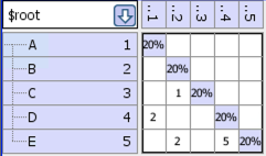
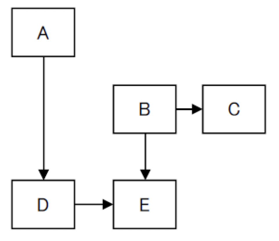
Example DSM
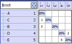
After we run the “disjoint” partitioner we get the following DSM, which shows the 2 disjoint sets:
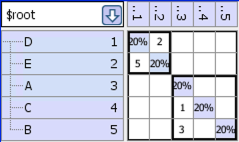
- For the example, the values are:
Number of edges = 4
Number of nodes = 5
Number of disjoint sets = 2
Path complexity = 4 – 5 + 2*2 = 3
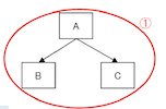
Similar to Cyclomatic Complexity, lower values are better. Here are some illustrating examples:
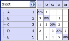
Good Example:
- Path complexity= E – N + 2*P= 4 – 5 + 2*1 = 1
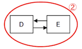
Bad Example:

- Path complexity= E – N + 2*P= 12 – 5 + 2*1 = 9
Many-to-Many Strength#
Other#
Violations#
The number of Design Rule Violations that exist within a subsystem.
Pagerank (not currently available)#
This metric measures the centrality of a system, by looking at the topology of the system dependency graph. Systems that are central have more impact on the architecture, even if they do not directly use/are not directly used by most systems. Unlike the above metrics, here we consider the dependency graph where the vertices are the selected partition and its siblings (systems that have the same parent as the selected partition). The PageRank of a vertex is proportional to the number of times it is visited in a very long random walk on the graph. Thus, the higher the PageRank of a system, the more central it is. After computing PageRank values we report the rank of each system, where the rank of s is n if there are n-1 systems with PageRank higher than that of s.
Clustering (not currently available)#
Measures how clustered the system dependency graph is, by calculating the average number of dependencies among elements used by each system. A higher clustering value indicates a more clustered system dependency graph. While some clustering is beneficial and reflects modular design, too much clustering is problematic because there are too many interdependencies among small subsets of systems.
Limits on Project Size and Overcoming the Limit#
Some of these metrics are computationally intensive, therefore we have set a limit on the size of the system dependency graph for their calculation. Some of the metrics are also dependent on the recursion limit of the Tarjan algorithm that is used for computing strongly connected components. This table lists the metrics to which the limits are applicable and the value of those limits:
Metric |
Applicable Size Limits |
System Stability |
15,000 atoms |
Average Impact |
15,000 atoms |
Connectedness |
15,000 atoms |
Connectedness Enrichment |
15,000 atoms, 40,000 dependencies |
Connectedness Strength |
15,000 atoms |
Coupling Enrichment |
15,000 atoms, 40,000 dependencies |
Coupling Strength |
15,000 atoms |
You can use View->Preferences->Metrics to force the computation of all metrics which have been limited by size. You can also increase the depth of the Tarjan recursion algorithm which can prevent Lattix from computing these metrics. Finally note that you may also have to increase the java stack size (specify -Xss1024k when you invoke Lattix) to avoid stack overflow due to recursion depth.
You also control a specific metrics to compute by setting a specific property. These properties are provided to override these size restrictions on the computation of metrics. To enable, set these properties to true in home/.lattix/lattix_username.properties file. Please note that the home directory is dependent on your operating system and your login name. The following properties are supported :
lattix.metrics.alwaysComputeMetrics: To force the computation of all metrics.
lattix.metrics.alwaysComputeImpact: To force the computation of AverageImpact and Stability Metrics.
lattix.metrics.alwaysComputeCumulativeDependency: To force the computation of Normalized Cumulative Dependency Metric.
lattix.metrics.alwaysComputeConnectedness: To force the computation of Connectedness Metric.
lattix.metrics.alwaysComputeConnectednessStrength: To force the computation of Connectedness Strength Metric.
lattix.metrics.alwaysComputeConnectednessEnrichment: To force the computation of Connectedness Enrichment Metric.
lattix.metrics.alwaysComputeCouplingStrength: To force the computation of Coupling Strength Metric.
lattix.metrics.alwaysComputeCouplingEnrichment: To force the computation of Coupling Enrichment Metric.
Please note that since the time for computation can be O(n^2) or O(n^3), bypassing the system size limit can make the CPU time used for computation unacceptably long.
Too much Recursion in Tarjan#
Metrics is compute intensive. Lattix uses the Tarjan’s graph algorithm for computing strongly connected vertices. Tarjan’s algorithm is the most efficient way to do this. It is a recursive algorithm. Lattix imposes a limit on the depth of recursion. It this limit is exceeded a message indicating excessive recursion depth is generated. You can override the limit in View->Preferences->Metrics or by setting the property:
lattix.dsmtools.max_tarjan=-1
This property can be added to the user’s property file in home/.lattix/lattix_username.properties file. Lattix should be closed before editing the property file. (Please note that the home directory is dependent on your operating system and your login name).
Metrics for Certain Well-known Systems#
Nant 0.85 |
Ant 1.7.1 |
ApacheServer 2.2.8 |
SpringSource 3.0 |
Eclipse 3.0 |
.NET Framework 2.0 |
|
|---|---|---|---|---|---|---|
Atom Count |
195 |
493 |
993 |
2165 |
3939 |
12308 |
Complexity |
0.02 |
0.12 |
0.62 |
1.78 |
11.9 |
165.84 |
System Stability |
72.4% |
91.47% |
95.82% |
98.81% |
91.22% |
93.02% |
Average Impact |
53.83 |
42.07 |
41.47 |
25.86 |
345.69 |
859.75 |
Internal Dependencies |
933 |
2386 |
6259 |
8223 |
30209 |
134740 |
Clustering |
8.92 |
7.18 |
20.84 |
2.64 |
15.96 |
46.94 |
Average Dependency |
4.78 |
4.84 |
6.3 |
3.8 |
7.67 |
10.95 |
Normalized Cumulative Dependency |
8.8 |
18.22 |
4.24 |
5.13 |
54.06 |
238.9 |
Connectedness |
29.66% |
29.31% |
3.73% |
2.34% |
15% |
24.43% |
Connectedness Enrichment |
0.76 |
0.54 |
0.2 |
0.05 |
0.2 |
0.3 |
Connectedness Strength |
22.99 |
41.29 |
18.98 |
16 |
137.2 |
645.16 |
Coupling |
6.22% |
9.17% |
0.07% |
0.01% |
1.58% |
2.95% |
Coupling Enrichment |
0.52 |
0.32 |
0.02 |
0 |
0.03 |
0.04 |
Coupling Strength |
1.02 |
2.75 |
0.09 |
0.02 |
3.66 |
20.15 |
System Cyclicality |
32.31% |
37.12% |
6.04% |
2.45% |
40.39% |
44.32% |
Intercomponent Cyclicality |
25.13% |
34.48% |
2.11% |
0% |
29.88% |
37.06% |
Object Oriented Metrics#
These metrics are available for object oriented languages and systems. At the moment, these metrics are supported for Java and .NET only. Note that these metrics are not supported for C/C++ simply because C/C++ software contains non-object oriented code constructs also (such as global methods and variables in files).
These are “package” or “directory” level metrics. It is also important to note that these metrics are computed by treating each package as external to each other. Thus package “a.b” is external to package “a.b.c” even though from a hierarchical standpoint “a.b.c” is contained within the package “a.b”.
Robert Martin Metrics#
Instability#
For this metric, the concept is that concrete implementations are inherently less stable than abstractions. That is, the more abstractions are used and depended on, the more stable a system will become. Conversely, the more concrete implementations are used and depended upon, the more unstable a system will become. Instability is calculated Outgoing Dependencies / (Outgoing Dependencies + Incoming Dependencies). This is the metric for Instability originally proposed by Robert Martin [1]. Calculated as
Instability = Outgoing Dependencies / (Outgoing Dependencies + Incoming Dependencies)
Abstractness#
This is a measure of how abstract is an implementation. In Software Engineering terms, this is a measure of the fractional number of atoms that are declared abstract, both pure abstract classes and abstract classes with some implementation. Abstractness is calculated Number of Interfaces and Abstract Classes / Atom Count; that is the Number of Interfaces and Abstract Classes / Number of Classes. This is the metric for Abstractness originally proposed by Robert Martin [1]. Calculated as
Abstractness = (Abstract Atom Count / Atom Count)
Distance#
The Distance metric is the distance from what is referred to as the Main Sequence on a graph of Abstractness versus Instability. The main sequence on that graph is a straight line starting at Abstractness=1, Instability=0 going to Abstractness=0, Instability=1. Distance is calculated as the absolute value of Abstractness + Instability -1. This is the metric for Normalized Distance originally proposed by Robert Martin [1]. Calculated as
Distance = |Abstractness + Instability -1|_ Outgoing Dependencies ^^^^^^^^^^^^^^^^^^^^^^^^^ Count of the number of “packages” that a “package” depends on. Note that the number does not depend on the number of actual dependencies between two packages, only that there is at least one dependency between them. This is the metric for Efferent Couplings originally proposed by Robert Martin [1].
Incoming Dependencies#
Count of the the number of “packages” that depend on a “package”. Note that the number does not depend on the number of actual dependencies between two packages, only that there is at least one dependency between them. This is the metric for Afferent Couplings originally proposed by Robert Martin [1].
Atom Count#
The number of Atoms, or leaf nodes for a system. What constitutes an Atom will be vary for different project types. Typically, this can be thought of as the number of compiled source code files that went into building the subsystem, but can be defined in a unique manner for a new dependency extraction plugin. For Java, the Atom Count is the number of classes inside a subsystem (inner classes are not in this count).
Abstract Atom Count#
The number of abstract classes inside my subsystem (inner classes are not in this count). Interfaces are treated as Abstract Atoms.