Applying Algorithms#
Lattix provides a range of algorithms that are useful for architecture discovery, analysis and refactoring:
Partitioning and Clustering Algorithms: Good for architecture discovery. Identify layers and components.
Restructuring Algorithms: Good for refactoring. Get suggestions on how to reorganize the system to improve modularity.
Other Algorithms: Identify critical dependencies.
Partitioning and Clustering Algorithms#
Lattix Architect provides a rich set of algorithms for architecture discovery and management. They help identify layering and componentization within the software system even after architectural intent has eroded. Large systems can be analyzed quickly by applying many of these algorithms and sharpening the understanding of the software system.
Partitioning Algorithms are applied using the Partitioning toolbar button:

Select a subsystem and mouseover the toolbar button to see which type of partitioning will be carried out by default. If you wish to choose a different type of partitioning, use the drop-down arrow adjacent to the Partitioning toolbar button:
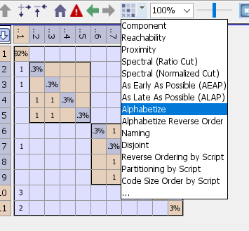
For full control over partitioning choices, click the drop-down arrow and then choose “…” to bring up the Partitioning Dialog:
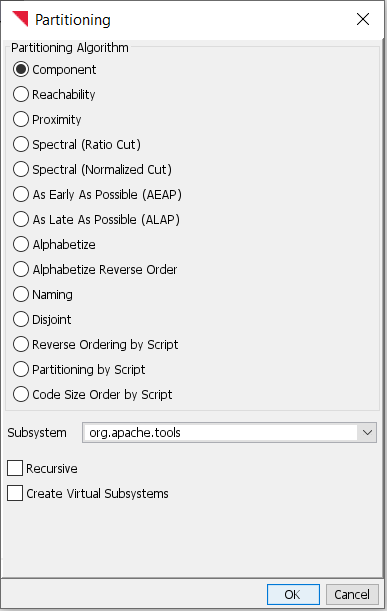
The Partitioning Dialog allows you to choose whether partitioning will happen recursively, for subsystems contained within the selected subsystem, or not. It also allows you to create subsystems for each of the virtual subsystems generated by the partitioning algorithm.
Partitioning Algorithms#
Component
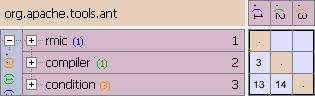
The Component partitioning algorithm groups strongly connected components into virtual partitions. In addition, independent subsystems are grouped together, as long as there are no cyclic dependencies between them. Within each virtual partition that is a strongly connected component, the subsystems are ordered to minimize the weight above the diagonal in the DSM. Once subsystems are grouped, topological sort is used to order them so that dependencies between the groupings go in the same direction.
Reachability
Reachability implements the Warfield algorithm for partitioning systems. It yields layers and independent subsystems just like the Component algorithm. However, it is significantly slower than the Component algorithm.
References
Details about the Warfield algorithm can be found here:
Warfield. Binary Matricies in System Modeling, IEEE Transactions on Systems, Management, and Cybernetics, Vol. 3, 1973.
Provider Proximity
Provider Proximity is a clustering algorithm that still produces a layered architecture. The providers are moved up as close as possible to the consumers.
As Early As Possible / As Late As Possible
These algorithms first group the systems into strongly connected components. They then create ordered layers with the property that the components in each layer are independent, and do not use any components in layers above. It is necessary to group the subsystems into strongly connected components first, because no layering is possible among the subsystems if there are dependency cycles. If the DSM represents dependencies between tasks, the components in each layer can be thought of sets of tasks that can be executed in parallel. The ALAP algorithm finds a layering such that each component is in the highest layer possible, while the AEAP algorithm finds a layering such that each component is in the lowest layer possible.
Instead of grouping the strongly connected components within each layer, we show these components as separate layers. The systems that are independent of each other (in this layer) also become their own layer. The layers (in this layer) are then ordered by size.
References
Cho. An Integrated Method for Managing Complex Engineering Projects Using the Design Structure Matrix and Advanced Simulation. MS Thesis, MIT, 2001.
Spectral
The Spectral partitioning algorithms are only applicable to systems with symmetric DSMs: whenever subsystem a uses subsystem b, it must be the case that b uses a also.
The Spectral partitioning algorithms order the elements such that those subsystems that are highly interdependent are put close to each other in the order. This ordering puts most of the dependencies close to the diagonal of the DSM and reveals the “block diagonal” structure of the matrix, where the blocks correspond to highly interdependent sets of subsystems. After applying the Spectral partitioning algorithms, the user can inspect the reordered matrix and group subsystems manually, or use the given virtual partitions. The virtual partitions break up the subsystems into two balanced sets, so that there are few dependencies between the sets. The Ratio Cut algorithm balances the two sets based on size, while the Normalized Cut algorithm balances the two sets using number of dependencies. One or both may be effective for a particular model.
References
Hagen and A. B. Kahng. New spectral methods for ratio cut partitioning and clustering. IEEE Transactions on Computer-Aided Design, 11(9):1074-1085, 1992.
Verma and M. Meila. A comparison of spectral clustering algorithms. Technical report, University of Washington, 2005.

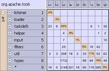
(A) An unorganized model.
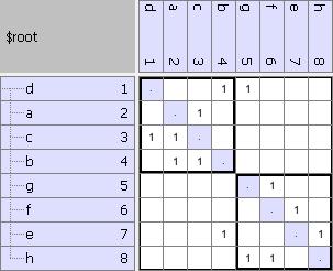
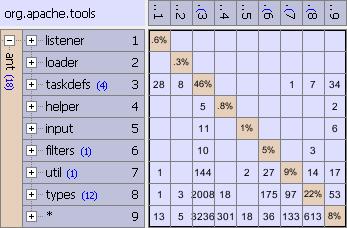
(B) Applying Ratio Cut to the model in (A). The new ordering reveals two components with few interdependencies.
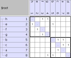
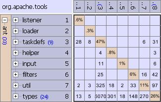
(C) Applying Normalized Cut to the model in (A). The groupings are the same as in (B), but the ordering is different.
Alphabetize
The partitions are listed alphabetically. This is the default organization when a project is first created.
Alphabetize Reverse Order
The partitions are listed in reverse alphabetical order.
Naming
The Naming partitioning algorithm creates parent partitions by grouping subsystems which have the same prefix. For instance, subsystems called xyz.c and xyz.h will be grouped under a parent partition called xyz.
Disjoint Subsystems
The Disjoint Subsystems partitioning algorithm finds disjoint components: members of each component do not use/are not used by members of any other component.
Other Options#
Recursive
Create Virtual Systems
Normally, the partitioning algorithm indicates the grouped partitions by bold squares within the DSM. If this option is selected, actual subsystems are created as parents for the grouped partitions.
Restructuring Algorithms#
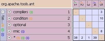
Very often, moving only a few partitions can result in a much cleaner architecture. For example, suppose that there is a dependency of subsystem A on subsystem B, which causes a dependency cycle in the architecture. However, if we look inside A and B, we see that this dependency is caused by a single partition a in A using a single partition b in B. Clearly, we can remove the top-level dependency by moving either a to B or b to A, cleaning up the top-level architecture. The following two algorithms use this intuition to clean up the architecture of the selected system by moving elements inside its subsystems. As an illustration, we apply them to the architecture below:
Reorganize System
Reorganize System moves children of subsystems of the selected system, in order to minimize the sum of weights of dependencies going “the wrong way” in the architecture. Here by “wrong way” we mean in reverse of the current ordering of the subsystems: any dependency A on B where A is listed before B. Because Reorganize System uses the ordering displayed in the DSM, it is best to apply a partitioning algorithm first, or manually order the subsystems consistent with architectural intent.
Dissolve Partition
Dissolve Partition is similar to Reorganize System, but it only moves elements in the selected subsystem S. It finds a new location for all the elements in S, moving each one to one of its siblings. As before, the objective is to minimize the sum of weights of dependencies going the wrong way in the architecture. Once all the elements are moved out of S, it is removed. Dissolve Partition should be applied to artificial subsystems, and is especially useful for * partitions in Java, because they contain classes not specified to be in any package.
Reorganize Labeled System
Reorganize Labeled System is similar to the two previous algorithms because it considers dependencies among the children of subsystems of the selected system. However, this algorithm creates new subsystems to group these elements, rather than simply rearranging them among the existing subsystems. The algorithm uses tags to help with the grouping, allowing the user to indicate elements which can be logically grouped together. The user may specify tags for individual elements, or tag an entire subsystem, which implicitly tags all of its children.
Reorganize Labeled System considers a dependency graph G, where the vertices are children of subsystems of the selected system. Some of these vertices have labels, corresponding to tags in the DSM. Reorganize Labeled System first finds the strongly connected components of G, creating a “component” graph, which is acyclic and where the vertices are the components. The algorithm then merges components with matching labels, as long as the new component graph has no cycles. The intuition behind this approach is that elements which are tagged with the same label belong together, as long as it does not introduce any new coupling in the architecture. After the merging is complete, the components are ordered using topological sort (such that all dependencies go in one direction). When the algorithm terminates, a subsystem is created for each component, which is named after its labels, and the original subsystems are removed. Moreover, inside the new subsystems elements are grouped into subsystems based on their original parents.
Hints for Removing Dependencies
You can also ask Lattix Architect to give you hints for removing a specific dependency in a cell. Simply, right click on a cell in the DSM to bring up the pop-up menu and select Hints for Removing Dependency. Lattix will compute the moves that could help to reduce the weight above the diagonal. Note that this assumes that the subsystems within the DSM for the selected system are organized in the desired order.
Other Algorithms#
Find Central Dependencies
This algorithm identifies dependencies that cause excessive coupling (cycles) in the selected subsystem. The removal of these dependencies splits up the strongly connected components of the architecture and reduces the weight above the diagonal of the DSM. Note that “no central dependencies can be found” will be reported if the subsystem to which the algorithm is applied does not contain cycles. This message may also be reported if no dependencies in the architecture stand out from the rest.
One way to use this algorithm is to combine it with Hide Dependencies. You can then repartition the the system to see what the structure would look like if some of the hidden dependencies are hidden.
Tag Cycles
This algorithm identifies all cycles within the selected subsystem. To see all cycles within the entire project, simply select $root and apply this algorithm. High level cycles such as cycles within packages are tagged HighLevelCycle while low level cycles such as cycles within classes are tagged LowLevelCycle. Cycles involving only member level elements are not tagged.